The rate of Earth’s rotation is not constant and this causes changes in the LOD²⁹. LOD changes (denoted by ΔLOD) occur over a broad range of timescales, from daily variations caused by tidal effects³⁰, to seasonal and annual changes caused mainly by atmospheric winds³¹ and to a gradual increase over millions of years caused by lunar tidal friction³². Fluctuations of several milliseconds (ms) also occur on timescales of 10–70 years, as shown in Fig. 1a between 1964 and 2019.

Full size image

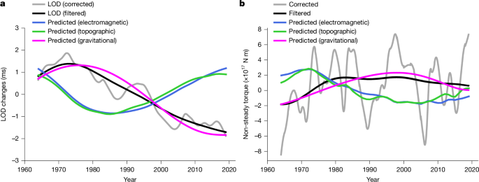
a, Observed decadal ΔLOD (in ms) between 1964 and 2019 (grey line) after removing the seasonal contributions from the atmosphere and oceans and the secular trends from lunar tidal friction, glacial isostatic adjustment and barystatic processes (Methods). The black line shows the multidecadal ΔLOD, obtained by applying a third-order low-pass Butterworth filter with a cut-off period of 30 years. b, The equivalent torque on the mantle (in N m) required to explain the decadal (grey line) and multidecadal (black line) ΔLOD. The blue, green and magenta lines are the predicted electromagnetic, topographic and gravitational torques, respectively (in b) and resulting multidecadal ΔLOD (in a) based on the ensemble solution of the core flow model from ref. ¹⁷ and inner core rotation time history from ref. ¹³, and with K_em = 1.0, K_top = 0.4, Γ = 1.3 × 10¹⁹ N m and τ = 6 years.

These decadal ΔLOD are the focus of our study. They are caused primarily by an exchange of angular momentum between the core and mantle. Flows near the top of the fluid core can be reconstructed from the observed secular variation of the geomagnetic field¹⁶. Predictions of the ΔLOD based on the angular momentum carried by these flows match the observed changes well^1,2,3, confirming their core origin.

However, the nature of the torque between the core and mantle responsible for these changes remains unclear. Core flows only exert a weak viscous stress on the CMB, too small to explain the required torque. Core flows also exert an electromagnetic stress on the electrically conducting mantle^4,5 and if a thin (several kilometres thick) layer of iron-enriched material is present at the base of the mantle with a conductance of G ≈ 10⁸ S, as suggested by studies of Earth’s nutations^33,34, electromagnetic coupling can produce a torque of the required magnitude^6,7. Predictions of the electromagnetic torque have been presented in several studies^5,9,35 and, although some correlations are observed, the match with the observed decadal ΔLOD is generally poor, unless core flows are specifically designed to match the required torque^6,7.

Pressure changes pushing laterally on topographic bumps of the CMB cause a so-called topographic torque on the mantle. Predictions based on the geostrophic pressure (reconstructed from core flows) and seismically derived maps of the CMB topography produce ΔLOD that are typically 100 times too large^8,9,10, highly sensitive to small changes in topography and core flows and the validity of this approach has been questioned³⁶. More recent modelling efforts instead focus on the pressure induced by the deflection of core flows over CMB bumps, in particular when the top of the core is stably stratified^37,38,39. No ΔLOD prediction based on this form of the topographic torque has yet been presented.

Decadal ΔLOD may also result from a gravitational torque by the inner core^11,12. On a time average, the topography of the inner core boundary (ICB) should coincide (except for a small eastward offset⁴⁰) with the gravitational potential imposed by mantle density anomalies. Time-dependent azimuthal (east–west) core flows exert electromagnetic stresses at the ICB rotating the inner core back and forth out of this longitudinal alignment, causing a fluctuating gravitational torque on the mantle^41,42. A prediction of this torque can be built given a time history of the changes in inner core rotation¹². However, only in recent years have such time histories been tentatively reconstructed on the basis of seismic observations^13,14,15,43.

We have known for more than 30 years—from an angular momentum budget approach—that the decadal ΔLOD are caused by core–mantle interactions^1,2. Yet we still lack a successful ΔLOD prediction based on a modelling of the torque on the mantle. On a long-term average, the mean westward flow at the CMB³ causes a westward torque on the mantle (from either electromagnetic or topographic coupling). This westward torque is balanced by a mean eastward gravitational torque from a slow, permanent eastward inner core rotation^12,42,44. Decadal ΔLOD result from fluctuations about this mean torque balance and here we build predictions of these fluctuations. Our reconstruction of the gravitational torque is based on the seismically inferred time history of inner core rotation changes from ref. ¹³, which only captures the broad multidecadal changes between 1964 and 2021. The core flow model¹⁷ that we use to reconstruct the electromagnetic and topographic torques at the CMB ends in 2019. Hence we restrict our attention to the time period 1964–2019 and focus our investigation on the multidecadal (about 60–70 years) ΔLOD (Fig. 1), rather than on the shorter decadal (about 10–30 years) variations.

We build predictions of the electromagnetic and topographic torques based on the probabilistic core flow model of ref. ¹⁷. The amplitude of the electromagnetic torque scales linearly with the mantle conductance, which we express in terms of a dimensionless conductance K_em (based on a reference value of 10⁸ S; Methods). The amplitude of the topographic torque depends on several parameters that are not well constrained and we express their collective influence in terms of a dimensionless factor K_top (Methods). Figure 1b shows the predictions of the electromagnetic and topographic torques based on the ensemble solution of the core flow model with K_em = 1.0 (that is, G = 10⁸ S) and K_top = 0.4. Although for these choices of K_em and K_top both torques are of the correct magnitude, their match to the required torque is poor and the ΔLOD that they predict are broadly opposite to those observed (Fig. 1a). Different choices of K_em and K_top change the amplitude but not the phase of the predicted torques. The latter is determined by the time history of core flows, mostly its large-scale part, and because the latter reproduces well the multidecadal ΔLOD (see Fig. 5 of ref. ³), it is well resolved by the secular variation.

The gravitational torque depends on a strength factor Γ and on the time history of the longitudinal misalignment (by an angle α) of the long equatorial axis of the ICB with respect to the degree 2 order 2 mantle mass anomalies (Methods). Changes in α result from changes in the bulk rotation of the inner core but the ICB topography also relaxes viscously with a characteristic time τ towards its equilibrium mantle alignment. The model of inner core rotation from ref. ¹³ that we use consists of a broad multidecadal oscillation with an amplitude of approximately φ ≈ 2.35° with respect to the mantle (Extended Data Fig. 1). The direction of rotation switches from prograde to retrograde in the vicinity of year 2010, as validated by other studies^14,15. With Γ = 1.3 × 10¹⁹ N m and τ = 6 years, the predicted gravitational torque matches both the amplitude and phase of the required torque and multidecadal ΔLOD (Fig. 1a,b). The good fit to the ΔLOD requires substantial viscous deformation of the ICB, shifting the time at which α (and the gravitational torque) is maximum to be around year 2000, instead of near 2010, as it would otherwise be for a rigid inner core.

The relative ease with which the gravitational torque can explain the multidecadal ΔLOD suggests that it is the main driver of these changes, at least within the time window 1964–2019, and, in turn, that the inner core rotation model from ref. ¹³ is broadly correct. The electromagnetic and topographic torques may play a role, but their opposite phase suggests that they act primarily to resist, not drive, the ΔLOD. Although the torque histories on Fig. 1 rest entirely on the accuracy of the models of inner core rotation and core flows, they are in line with results from dynamo simulations approaching Earth-like conditions that suggest a similar scenario of gravitationally driven multidecadal ΔLOD opposed by a CMB torque¹⁸.

The gravitational torque history in Fig. 1 is based on a specific set of Γ and τ, but equally good fits to the ΔLOD are achieved for a range of these parameters, as well as for a range of K_em and K_top if electromagnetic and topographic coupling contribute to resisting a part of the gravitational torque. We now proceed to determine the best-fit values of these parameters, none of which are well known, through a Bayesian inversion. We consider a scenario in which the total torque on the mantle results from the sum of the gravitational and either the electromagnetic or topographic torque. In reality, both of these CMB torques act jointly, but given the similarities of their time histories, a trade-off between a higher K_em and a lower K_top (or vice versa) produces similar ΔLOD predictions. It is then easier to consider these torques separately for results tractability and to establish upper bounds on K_em and K_top individually.

We compute ΔLOD predictions for a large number of individual samples, each consisting of a specific combination of Γ, τ and K_cmb, in which K_cmb is either K_em or K_top. Our sampling scheme is based on a Markov chain Monte Carlo (MCMC) algorithm (Methods). To cover the uncertainty in core flows, for each sample, we select randomly one of 400 different realizations of the model in ref. ¹⁷ and compute its associated electromagnetic and topographic torques (Extended Data Fig. 2). Likewise, for each sample, we select randomly an inner core rotation history that falls within the bounds of the model in ref. ¹³ (Extended Data Fig. 1).

Figure 2a–c shows the posterior distributions of Γ, τ and K_em for the samples that provide the most successful ΔLOD fit (a misfit χ < 0.2 ms; Methods) when the CMB torque is from electromagnetic coupling (the posterior distributions for all samples are shown in Extended Data Fig. 3). From this subset of samples, we find maximum a posteriori (MAP) estimates of Γ = 1.4 × 10¹⁹ N m, τ = 10.2 years and K_em = 1.08 (that is, G = 1.08 × 10⁸ S). The 95% confidence interval (CI) for each are: Γ ∈ [0.6–2.2] × 10¹⁹ N m, τ ∈ [4.1, 30.5] years and K_em ∈ [0.05, 2.89] (Extended Data Table 1). The predicted ΔLOD and the time histories of the gravitational, electromagnetic and total torques are shown in Fig. 3a–c. All samples with χ < 0.2 ms fit the multidecadal ΔLOD very well. The gravitational torque is generally in phase with the total torque; it drives the ΔLOD and is larger than the electromagnetic torque, which opposes the gravitational torque. Viscous relaxation of the ICB limits α to be <2° and shifts the timing of its maximum positive eastward offset to occur near year 2000 (Extended Data Fig. 4). We find two asymptotic torque regimes (Supplementary Information): one in which the gravitational torque explains the ΔLOD largely by itself and the other featuring large and opposed gravitational and electromagnetic torques as observed in Earth-like dynamo simulations¹⁸. The best ΔLOD fits occur at the intersection of these two regimes, with the gravitational torque larger than the electromagnetic torque by a factor between 1 and 2.

Full size image

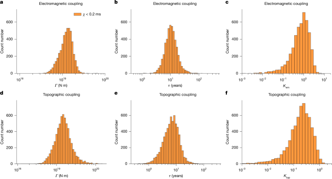
a–c, Γ, τ and K_em when the CMB torque is from electromagnetic coupling. d–f, Γ, τ and K_top when the CMB torque is from topographic coupling. Only the high-probability samples for which the ΔLOD misfit χ is <0.2 ms are included.

Full size image

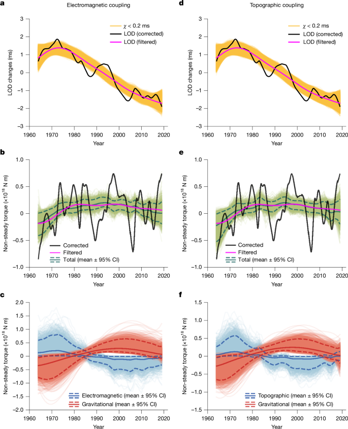
a,d, ΔLOD predictions from high-probability samples (χ < 0.2 ms, yellow lines) compared with the decadal ΔLOD (black line) and multidecadal ΔLOD (magenta line). b,e, Predictions of the total torque (thin green lines) for high-probability samples compared with the decadal (black line) and multidecadal (magenta line) torque required to produce the ΔLOD. c,f, Predictions of the gravitational (thin red lines) and CMB torque (thin blue lines) for the high-probability samples. In b,c,e,f, thick solid coloured lines indicate the median of the torque histories and dashed lines enclose the region containing the 95% CI.

Figures 2d–f and 3d–f show the results when the torque at the CMB is instead caused by topographic coupling. The fit to the ΔLOD is equally good, with the gravitational torque slightly more dominant. The 95% CI range of Γ that provides the best ΔLOD fit is shifted to higher values (Γ ∈ [0.6–4.2] × 10¹⁹ N m, a MAP estimate of 1.5 × 10¹⁹ N m) but the range of τ is shifted to smaller values (τ ∈ [1.7–21.5] years, a MAP estimate of 7.8 years), such that the product Γτ remains approximately unchanged. We find K_top ∈ [0.01–0.83] with a MAP estimate of 0.23.

The torque histories (Fig. 3) confirm the dynamical picture inferred from the individual realizations (Fig. 1); the broad, approximately 70-year oscillation in inner core rotation drives a gravitational torque that is dominantly responsible for the multidecadal ΔLOD, whereas the torque at the CMB acts to resist these changes. This relatively simple oscillating torque history on the mantle is supported by the changes in zonal core flows at the CMB over the past seven decades (Fig. 4a and Supplementary Information). For about 35 years centred on 1967, the zonal flows inside the tangent cylinder were more westward than on average (although this reflects mostly the flow in the Northern Hemisphere). If axially invariant, such flows entrained (through electromagnetic coupling at the ICB) a westward rotation of the inner core, leading to a westward misalignment α of its long equatorial axis and a westward gravitational torque on the mantle (Fig. 4b). Over the same time period, the zonal flow outside the tangent cylinder was eastward, exerting an eastward torque at the CMB. For the next 35 years (centred on 2002), the flow structure was reversed (Fig. 4a,c). These oppositely directed zonal flows, inside and outside the tangent cylinder, switching directions over a roughly 70-year period, are ultimately responsible for the observed multidecadal ΔLOD. Whether this flow structure is periodic, and repeats over time, or whether it only reflects the dynamics over the past seven decades, is unknown. Core flows in 1915–1949 show hints of resemblance to the 1985–2019 structure but also some notable differences (Extended Data Fig. 5) and the quality of the secular variation that far back in time may not be good enough to draw robust conclusions.

Full size image

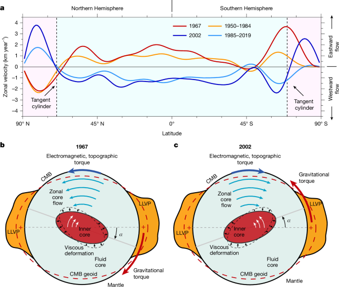
a, Differential zonal azimuthal core flow versus latitude at the CMB in 1967 (red line), 2002 (dark blue line), time-averaged over 1950–1984 (orange line) and over 1985–2019 (light blue line), all with respect to the time-averaged flows between 1950 and 2019, from the ensemble solution of the core flow model in ref. ¹⁷. Pale pink highlights the regions inside the cylinder tangent to the equator of the inner core (the tangent cylinder); pale cyan highlights the region outside the tangent cylinder. A positive (negative) zonal flow is more eastward (westward) compared with its mean time average. b,c, Equatorial cross-section schematics of the core flows and torques in 1967 and 2002. Light blue arrows depict the zonal core flow outside the tangent cylinder with respect to its mean time average; white arrows depict the mean of the zonal core flow near the ICB above and below the inner core inside the tangent cylinder. Thick dark red and dark blue arrows indicate the directions of the gravitational and CMB torques, respectively. The longitudinal misalignment α of the long equatorial axis of the inner core with respect to its equilibrium alignment with the CMB geoid (dashed red ellipsoid) results from the combined effects of differential rotation and viscous relaxation (small black arrows). The amplitudes of the elliptical CMB geoid and ICB topography are greatly exaggerated for ease of visualization. We assumed for the purpose of the illustration that the equatorial CMB geoid (positive mantle mass anomalies, depicted by the red ‘+’ signs) is longitudinally aligned with the LLVPs in the lower mantle, but this may not be the case, and our results are independent of this alignment.

Our reconstructed multidecadal torque scenario is supported by the seismically inferred inner core rotation changes, by zonal core flows derived from the secular variation and by dynamo simulations. However, our estimates of Γ, τ and K_cmb are only as accurate as the models of inner core rotation and core flows that we used. These models contain several assumptions, which map into an uncertainty on our retrieved torque parameters. Sensitivity tests (Supplementary Information) show that an increase (decrease) in the amplitude of the inner core differential rotation leads to a proportional decrease (increase) in Γ and that the best-fit estimate of each torque parameter can vary by up to 30% for different core flow models.

Although the specific numerical values of the torque parameters that we retrieve remain uncertain, their scales have important geophysical implications for the deep mantle and inner core. Γ provides a measure of the magnitude of the degree 2 order 2 () topography of the geoid at the CMB^11,45, which, in turn, depends on the structures, dynamics and material properties of the lowermost mantle. Our best-fit range of Γ = [0.6–4.2] × 10¹⁹ N m (when combining the results of electromagnetic and topographic coupling) is lower than a previous estimate⁴⁵ and implies a peak-to-peak CMB geoid topography of about 31–83 m and a corresponding ICB topography of about 11–29 m (although both estimates depend on the density contrast at the ICB; Methods). Numerical models of mantle convection⁴⁶ can reproduce such low CMB geoid values (Extended Data Fig. 6) but only when two key dynamical elements are included: (1) large low-velocity provinces (LLVPs) in the lowermost mantle must consist of thermochemical piles of distinct (and intrinsically denser) material that are also warmer, such that their effective density is near-neutral, as supported by a several lines of evidence^19,20,21; (2) a pPv phase that has a weaker viscosity (by 2 to 3 orders of magnitude) than the bridgmanite phase, as supported by mineral physics²². The low Γ that we retrieve is then consistent with, and provides tentative support for, chemically distinct LLVPs and a pPv phase with a low viscosity.

The viscous relaxation time of the inner core that we find, in the range 2–31 years, implies a viscosity of 10¹⁷–10¹⁸ Pa s if uniform, or smaller, 10¹⁵–10¹⁶ Pa s, if confined to the top part of the inner core⁴⁰. Such values are in agreement with recent estimates based on laboratory experiments^26,27, ab initio molecular dynamics calculations²⁸ and the attenuation of seismic shear waves within the inner core⁴⁷.

If the CMB torque is dominated by electromagnetic coupling, our best-fit mantle conductance is G = 1.08 × 10⁸ S, although it may be lower if the short-wavelength (and unresolved) CMB magnetic field contributes to a substantial part of the electromagnetic torque⁴⁸. Our retrieved G is consistent with the observed attenuation of Alfvén waves travelling across the fluid core⁴⁹. The electrical conductivity of (Mg,Fe)O at CMB conditions is in the range 10⁴–10⁵ S m⁻¹ (refs. ^23,24), so a thin (approximately 2-km) global layer of dense, iron-enriched material at the base of the mantle, consistent with inferences from seismic normal modes²⁵, is compatible with our findings. Notably, our results also place an upper bound of G ≤ 2.9 × 10⁸ S, which limits the possible thickness of this layer, consistent with the limited time delay of geomagnetic signals propagating through the mantle⁵⁰.

Alternatively, if topographic coupling dominates the CMB torque, our upper bound of K_top ≤ 0.83 places a limit on the buoyancy frequency N of the stratification (whether thermal or compositional) at the top of the fluid core (Methods). It is difficult to place a strict upper bound on N (Supplementary Information) but our results point to a value smaller than Earth’s rotation frequency Ω_o, and ≪ Ω_o if electromagnetic coupling is responsible for a large fraction of the CMB torque. This is in line with dynamo models, which also require a small N to match the characteristics of the observed secular variation¹⁸.

Our results indicate that the multidecadal ΔLOD are driven by small differences between the (leading) gravitational and (resisting) CMB torques. These two torques must be in balance on a long-term average^12,42,44 and our best-fit torque parameters imply a small permanent eastward misalignment of 1.2° between the ICB topography and the CMB geoid, and a steady eastward differential inner core rotation of 0.12° year⁻¹ (Methods). Our ΔLOD prediction is limited to the broad multidecadal changes primarily because of the limited temporal resolution of the seismically inferred inner core rotation history. However, the short τ ≈ 10 years that we retrieve implies that the gravitational torque is inefficient at periods shorter than a few decades¹⁸ and, consequently, that the decadal (10–30 years) and shorter core-induced ΔLOD are probably driven by the CMB torque (Supplementary Information). Yet, the predicted electromagnetic and topographic torques do not contain large decadal fluctuations (Fig. 1). This may reflect the limited resolution of the core flow model or indicate that models of CMB coupling need refining. As our study illustrates, better explaining the nature of the core–mantle torque driving the ΔLOD contributes to sharpening our understanding of the structures, material properties and dynamics in the deep interior of Earth.

Torque and changes in the LOD

An axial torque Γ_z acting on the mantle causes a change in its rotation rate (ΔΩ_m) according to

in which C_m = 7.13 × 10³⁷ kg m² is the axial moment of inertia of the mantle. ΔΩ_m corresponds to a change in the LOD (ΔLOD)

in which Ω_o = 2π/86,400 s⁻¹ is the reference mantle rotation rate based on a 24-h day length. The equivalent torque causing the observed ΔLOD can therefore be reconstructed from

The decadal ΔLOD (grey line in Fig. 1) between 1964 and 2019 are obtained after removing the LOD contributions from the atmosphere, oceans, lunar tidal friction, glacial isostatic adjustment and barystatic processes at Earth’s surface (Extended Data Fig. 7). The multidecadal ΔLOD (black line in Fig. 1) are obtained by applying a third-order low-pass Butterworth filter with a cut-off period of 30 years to the decadal ΔLOD signal (Extended Data Fig. 8). More details on these operations are provided in the Supplementary Information.

We build predictions of ΔΩ_m (and ΔLOD) from

by numerically integrating in time from 1964 to 2019 forward models of the torque from surface forces at the CMB (Γ_cmb) and the gravitational torque from the inner core (Γ_g). We consider two different sources of Γ_cmb, electromagnetic and topographic coupling. Multidecadal ΔLOD result from fluctuations in the torque on the mantle about a mean balance^12,42,44. To focus on these, we subtract a temporal mean from all of our predictions of gravitational, electromagnetic and topographic torques.

Electromagnetic torque

The axial electromagnetic torque can be written as a surface integral over the (assumed spherical) CMB as^4,5,6

in which r_c = 3,485 km is the radius of the core, μ is the magnetic permeability of free space, B_r and B_ϕ denote the radial and azimuthal components of the magnetic field, respectively, and dS is a surface element, θ is co-latitude and ϕ is longitude. Predictions of the temporal variations of Γ_em depend on models of how B_r and B_ϕ change with time at the CMB.

The magnetic field at the CMB can be decomposed as \({\bf{B}}=\nabla \times \nabla \times {\mathcal{S}}{\bf{r}}\,+\) , in which r is the radial vector and and are poloidal and toroidal scalar fields, respectively. B_r only involves , whereas B_ϕ involves both and . Consequently, we can separate Γ_em into its poloidal and toroidal contributions to B_ϕ (refs. ^5,6).

The poloidal part of Γ_em can be reconstructed directly from magnetic field models built from observations. Such models provide time-dependent maps of at the Earth’s surface, which are down-continued to the CMB. For a thin layer of conducting mantle material above the CMB with conductance G, the poloidal torque is^5,6

in which and are the Gauss coefficients of the field model (with l and m the spherical harmonic degree and order, respectively), and are their time derivatives and r_e = 6,371 km is Earth’s radius.

The toroidal part of Γ_em is given by

in which includes contributions from the diffusion of the toroidal field at the top of the core into the conducting mantle and from the advection of the radial field by the flow v tangential to the CMB. We assume that the latter contribution dominates (see ref. ⁶), in which case we can write

in which \({L}^{2}=-[\frac{1}{\sin \theta }\frac{\partial }{\partial \theta }\left(\sin \theta \frac{\partial }{\partial \theta }\right)+\frac{1}{{\sin }^{2}\theta }\frac{{\partial }^{2}}{\partial {\phi }^{2}}]\) is the angular momentum operator and ∇_H is the surface gradient. Evaluation of this torque requires both a time-dependent model of the magnetic field (to evaluate B_r) and a time-dependent model of tangential flow v at the CMB. Models for v, in turn, are built such that they are compatible with the observed secular variation of the magnetic field¹⁶.

The total electromagnetic torque Γ_em is the sum of and and is proportional to the mantle conductance G, which we leave as a free model parameter to be determined. We write G = K_emG_ref, in which G_ref is a reference conductance set equal to 10⁸ S. For given magnetic field and flow models, the strength of the electromagnetic torque scales with the dimensionless conductance K_em.

Our predictions of Γ_em are based on the magnetic field model COV-OBS.x2 (ref. ⁵¹) and the probabilistic core flow model from ref. ¹⁷. These predictions are shown in Extended Data Fig. 2 and lead to multidecadal ΔLOD predictions that are broadly reversed compared with that observed (Fig. 1). The poor ΔLOD match may be because core flows are not sufficiently well resolved. Indeed, core flow models may be designed such that, as well as matching the observed secular variation, they also generate an electromagnetic torque that matches the observed ΔLOD (refs. ^6,7). The required flow adjustment tends to be small. However, although this small adjustment is not in conflict with the secular variation, it is also not required by it. Synthetic tests using numerical dynamo models show that the large-scale core flows retrieved from the secular variation contribute the most and provide an adequate prediction of the electromagnetic torque⁴⁸. This suggests that the electromagnetic torque prediction built from large-scale core flows should be broadly correct and that the mismatch with the observed ΔLOD of Fig. 1 indicates instead that electromagnetic coupling at the CMB is not the dominant multidecadal torque on the mantle. Synthetic tests⁴⁸ also suggest that the small length scales of the CMB magnetic field (l > 13), inaccessible from observations, may contribute to about a third of the total electromagnetic torque. Our reconstruction of the electromagnetic torque may then be underestimated, contributing to an overestimate in our recovered value of G.

We assume a uniform conductance G in the mantle. Although the bottommost region of the mantle (the D″ region) is most likely heterogeneous, and electrical conductivity is expected to vary with geographic position, the precise way in which it does is unknown, so the simplest approach is to assume a uniform G. Using a non-uniform G can modify the time history of the electromagnetic torque⁵² and can thus alter our inversion results for the best-fit torque parameters. However, we consider it unlikely that the geometry of G could reverse the sign of Γ_em and account for most of the multidecadal ΔLOD on its own.

Topographic torque

The topographic torque Γ_top results from the dynamic pressure associated with core flows acting on the CMB topography. Recent modelling efforts^37,38,39 focus on the perturbation in the pressure field that is induced by the deflection of a mean tangential flow by CMB bumps in a stratified fluid with buoyancy frequency N and permeated by a magnetic field of strength B₀. The axial component of Γ_top can be written as

in which T_ϕ is the azimuthal stress on the CMB. Idealized models of T_ϕ can be developed for a steady and uniform azimuthal flow v_ϕ acting on a localized region of the CMB with a periodic topography of wavelength ℓ and amplitude h. The model in ref. ³⁹ relates T_ϕ to v_ϕ as

in which \({\rm{sign}}({v}_{\phi })=\frac{{v}_{\phi }}{\parallel {v}_{\phi }\parallel }\),

and ρ is the fluid density, η is the magnetic diffusivity and F(θ) is a function of co-latitude that takes into account the projection of the Coriolis force with the normal to the boundary (Extended Data Fig. 9). The parameter has units of kg m^−3/2 s^−3/2 and incorporates a collection of physical parameters that influence the torque. Some of these parameters (ρ, η, B₀) are reasonably well known, but N is not, and we lack a detailed model of the CMB topography, so h and ℓ are also not well constrained. To take into account different possible values of , we write it as , in which K_top is a dimensionless parameter and is a reference value of set equal to 1 kg m^−3/2 s^−3/2. The topographic torque from equation (9) can then be written as

The time history of Γ_top depends on the time history of v_ϕ. For a given flow model at the CMB, K_top modulates the amplitude of the topographic torque and is a parameter left to be determined. Its numerical value provides a constraint on N for the chosen values of h and ℓ (Supplementary Information).

Predictions of Γ_top based on the flow model in ref. ¹⁷ are shown in Extended Data Fig. 2. By itself, Γ_top does not generate the multidecadal ΔLOD that match observations (Fig. 1). Notably, the Γ_top model that we used is highly idealized; it is based on a steady and uniform flow at different points of the CMB, whereas the true flow is time-dependent and laterally varying. Moreover, we assume for simplicity that is uniform but it probably has lateral variations. Allowing to vary with position at the CMB would change the time variations of this prediction. However, the general trend of Γ_top follows that of Γ_em and illustrates that, to the first order, both of these torques depend on the fluctuations of the large-scale v_ϕ flow at the CMB; when v_ϕ is generally westward (eastward) compared with its mean time average, the tangential stress on the CMB from either electromagnetic or topographic coupling is also westward (eastward).

Gravitational torque

The gravitational torque on the mantle Γ_g is given by¹¹:

in which Γ is a strength factor and α is the longitudinal angle of the degree 2 order 2 (long equatorial axis) topography of the inner core with respect to the gravitational potential imposed by mantle mass anomalies. The evolution of α depends on the bulk axial angular rotation angle φ of the inner core (related to the differential inner core angular velocity Ω_i by ) and the viscous relaxation time τ for the ICB topography to realign with its equilibrium shape,

We use a time history model of φ based on the seismic reconstruction from ref. ¹³ (Extended Data Fig. 1). Predictions of Γ_g depend on the time history of α, which is computed by integrating numerically equation (14) for our model of φ and a given choice of τ. Note that equation (14) describes the change in α with respect to a permanent offset α_o associated with the long-term torque balance on the mantle.

In the limit of τ ≪ T/2π, when viscous relaxation of the ICB occurs rapidly compared with the nominal multidecadal period of T ≈ 70 years of inner core rotation changes, \(\frac{{\rm{d}}\alpha }{{\rm{d}}t}\ll \alpha /\tau \), so that, from equation (14), \(\alpha \approx \tau \frac{{\rm{d}}\varphi }{{\rm{d}}t}=\tau {\varOmega }_{{\rm{i}}}\), and Γ_g can be approximated as

In this limit, Γ_g constrains the product of Γ and τ, not their individual values.

The strength factor Γ is related to the amplitude of the degree 2 order 2 geoid at the CMB (specified in terms of a spherical harmonic coefficient ) by^45,53

in which r_i = 1,221 km is the ICB radius, g_i = 4.4 m s⁻² is the gravitational acceleration at the ICB, ρ_i is the inner core density (assumed uniform) and ρ_f is the density of the fluid core at the ICB. The peak-to-peak topography of the geoid along the equator of the CMB, , is related to by \({h}_{2}^{2}=2\sqrt{\frac{45}{96{\rm{\pi }}}}{U}_{2}^{2}=0.7725{U}_{2}^{2}\).

To convert Γ to , we use ρ_i = 12,730 kg m⁻³ and ρ_f = 12,160 kg m⁻³ based on the preliminary reference Earth model (PREM)⁵⁴. However, the density contrast at the ICB remains not well constrained and may be as high as 600–900 kg m⁻³ (ref. ⁵⁵) or as low as 200–300 kg m⁻³ (ref. ⁵⁶). This uncertainty on ρ_i and ρ_f maps to an uncertainty on the CMB geoid inferred from Γ. Using PREM, our range of Γ ([0.6–4.2] × 10¹⁹ N m) corresponds to a range of at the CMB of 31–83 m. The gravitational potential anomaly of degree 2 varies approximately linearly with radius inside the core^45,53, so the peak-to-peak topography along the equator of the ICB (assumed to coincide with an equipotential surface) is \(({r}_{{\rm{i}}}/{r}_{{\rm{c}}}){h}_{2}^{2}\approx 0.35{h}_{2}^{2}\), corresponding to a range of peak-to-peak ICB topography of 11–29 m. Although small, an axial rotation of this topography by about 1° (Extended Data Fig. 4) is sufficient to provide the necessary gravitational torque on the mantle. Our results indicate that viscous relaxation of this ICB topography occurs over a timescale of around 10 years (Extended Data Fig. 4), amounting to radial motion on the order of 10 m near the top of the inner core. It is unclear whether such a small-amplitude (and low-wavelength) displacement can be detected seismically or whether seismic inferences of viscous deformation near the top of the inner core⁵⁷ capture instead a more regional deformation.

Torque balance

Palaeomagnetic observations⁵⁸ suggest that the present-day mean westward differential flow at the CMB has persisted for the past 9,000 years, at a mean rate of Ω_w = 0.09° year⁻¹. This mean flow produces a mean westward torque on the mantle, from either electromagnetic or topographic coupling or a combination of both. On a long-term average, this torque is balanced by an eastward gravitational torque maintained by a steadily differentially rotating and viscously deforming inner core^{12,40,42,44,59}. Assuming that the CMB torque is caused by electromagnetic coupling, a measure of the steady westward electromagnetic torque is given by^44,59

in which \({\bar{B}}_{{\rm{r}}}=0.4\,{\rm{mT}}\) is the root mean square strength of the radial magnetic field at the CMB and K₁ = 2.3 is a numerical factor. A balance between Γ_w and the gravitational torque (equation (13)) implies a permanent eastward angular offset of

Using our best-fit Γ (= 1.4 × 10¹⁹ N m) and G (= 1.08 × 10⁸ S) gives α_o = 1.19°. From equation (14), the steady (dα/dt = 0) eastward differential inner core rotation associated with this offset is Ω_i = α_o/τ and our best-fit estimate of τ (= 10.2 years) gives Ω_i = 0.12° year⁻¹, equivalent to that found in dynamo models at Earth conditions¹⁸. Such a rate would account for a substantial part of the observed differential rotation of the inner core (Extended Data Fig. 1) and implies that, over the past 9,000 years over which the westward drift has persisted, the inner core has undergone close to three full rotations with respect to the mantle.

Inversion of torque parameters

We retrieve the set of torque parameters (Γ, τ, K_cmb), in which K_cmb is either K_em or K_top, that best fit the observed ΔLOD based on a Bayesian framework^60,61. We define the probability of a sample θ ≡ θ(Γ, τ, K_cmb) as

in which

is the root mean square misfit between the predicted (ΔLOD_pre(θ)) and observed (ΔLOD_obs) changes in LOD at times t_i over the period 1964–2019 using a one-year sampling interval (N_s = 56). σ is the standard deviation associated with the low-pass-filtered multidecadal ΔLOD signal. Its numerical value is arbitrary; we use σ = 0.2 ms, which gives a reasonable compromise between ensuring a good fit to the multidecadal ΔLOD while allowing for some uncertainty in its reconstruction.

To sample the parameter space of θ and build posterior distributions of Γ, τ and K_cmb, we use an adaptive MCMC algorithm^60,61. For a current state of the chain θ_n, the distribution of a proposed sample θ* is multivariate normal and specified by

in which Σ_n is the covariance matrix and s is the step size. For each proposed sample of torque parameters, we randomly select one of the 400 core flow realizations to build a prediction of either Γ_em or Γ_top, which is then multiplied by K_em or K_top, respectively. We also randomly select a time history of the inner core rotation angle φ that falls within the bounds of the model of ref. ¹³ and compute Γ_g from equations (13) and (14) based on the values of Γ and τ of the present sample. The ΔLOD prediction from these is then computed from equation (4). The acceptance of a proposed sample is based on a Metropolis–Hastings algorithm: if π(θ*) ≥ π(θ_n), the proposed sample is accepted; if instead π(θ*) < π(θ_n), a random number u is drawn between 0 and 1, and if u ≤ π(θ*)/π(θ_n), the proposed sample is accepted; otherwise, it is rejected.

Our adaptive strategy comprises two parts. First, the covariance matrix Σ_n is iterated over the accepted samples following a recursive scheme based on the Welford algorithm⁶². Second, we adaptively tune the step size s, which controls the exploration efficiency of the Markov chain. We update s every 1,000 iterations based on the recorded acceptance rate (the ratio of accepted to total proposed samples) to maintain it within an empirical optimal range of 0.05–0.15. Both Σ_n and s are adapted during the first 10,000 samples of the burn-in phase (which consists of 20,000 samples). Their values are kept fixed for subsequent samples.

Our final distributions are compiled by combining five independent chains started from a dispersed set of initial guesses (Supplementary Information). Each chain consists of 180,000 samples generated after the burn-in phase. To reduce the autocorrelation between draws, we thin the output of every chain by storing only every tenth draw. This results in 18,000 samples per chain and a total of 90,000 posterior samples. The convergence of our distributions were tested on the basis of standard MCMC performance metrics (Supplementary Information).

The datasets generated as part of this study, together with the Python scripts and data files necessary to reproduce all figures, are freely accessible on Borealis at https://doi.org/10.5683/SP3/RA3KHX. The core flow and magnetic field models are available from the pygeodyn website at https://geodyn.univ-grenoble-alpes.fr/.

The software package related to MCMC performance metrics is available at ArviZ (https://python.arviz.org/en/stable/).

We thank Y. Yang and X. Song for sharing their inner core rotation model and F. Deschamps for sharing with us the CMB geoid computed on the basis of his previous mantle convection results. We also thank P. Koelemeijer and G. Soldati for sharing their CMB topography models. The comments and suggestions by R. Holme and two anonymous reviewers greatly improved our study. H.Z. acknowledges support from the Roy Dean Memorial Scholarship and Roy Dean Hibbs Memorial Travel Award from the Institute for Geophysical Research at the University of Alberta.

H.Z. and M.D. disclose support for the research of this work from the Natural Sciences and Engineering Research Council of Canada (grant numbers RGPIN-2018-0596 and RGPIN-2025-05158).

1. These authors contributed equally: Huifeng Zhang, Mathieu Dumberry

Authors and Affiliations

1. Department of Physics, University of Alberta, Edmonton, Alberta, Canada

   Huifeng Zhang & Mathieu Dumberry

M.D. acquired the funding, designed the study and developed the preliminary model. H.Z. performed the numerical tests. Both authors contributed to figures preparation, geophysical analysis and writing of the manuscript.

Corresponding authors

Correspondence to Huifeng Zhang or Mathieu Dumberry.

Competing interests

The authors declare no competing interests.

Peer review information

Nature thanks Dominique Jault, Paolo Personnettaz and the other, anonymous, reviewer(s) for their contribution to the peer review of this work. Peer reviewer reports are available.

Publisher’s note Springer Nature remains neutral with regard to jurisdictional claims in published maps and institutional affiliations.

Open Access This article is licensed under a Creative Commons Attribution-NonCommercial-NoDerivatives 4.0 International License, which permits any non-commercial use, sharing, distribution and reproduction in any medium or format, as long as you give appropriate credit to the original author(s) and the source, provide a link to the Creative Commons licence, and indicate if you modified the licensed material. You do not have permission under this licence to share adapted material derived from this article or parts of it. The images or other third party material in this article are included in the article’s Creative Commons licence, unless indicated otherwise in a credit line to the material. If material is not included in the article’s Creative Commons licence and your intended use is not permitted by statutory regulation or exceeds the permitted use, you will need to obtain permission directly from the copyright holder. To view a copy of this licence, visit http://creativecommons.org/licenses/by-nc-nd/4.0/.

Reprints and permissions